INVESTIGATING THE EFFECT OF GLUCOSE CONCENTRATION
ON THE RATE OF REPRODUCTION OF YEAST CELLS
Prediction
In this section I will look at all the factors involved
in the rate of reproduction of yeast cells, bring them together at the end of
the section and deduct a scientific conclusion as to what I would expect to
happen.
Yeast Cell Respiration
Yeast cells, like any other organism, need a substrate to
respire.
Respiration in general
In respiration, they use the substrate to produce ATP for cell metabolism. The overall equation for respiration using glucose is:
C6H12O6 + 6O2 Þ 6CO2 + 6H2O
 Therefore, the more glucose available, the
greater the rate of respiration and the easier it is for cell metabolism to
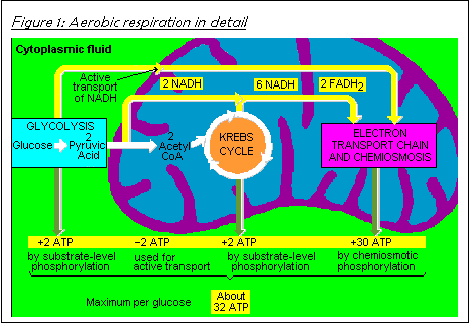
take place. The more detailed version
of the respiratory pathway is shown in Figure
1. However, one cannot merely
assume that a greater rate of respiration can occur with a higher level of
glucose concentration because it is a living organism involved. This means that high levels of glucose
concentration could cause the yeast cells to become crenated and therefore the
reproductive mechanisms would not function because of the physiological strain
caused by the low pressure potential.
This would mean that the initial rate of reproduction would be much less
than that of cells in solutions of glucose concentrations on the limit of the
cell’s pressure potential. However,
this need not be a worry because I will not use glucose of such a high concentration.
Also, because it is an organism, other factors like waste products and method
of uptake need to be taken into account. These are discussed below.
Glucose catabolism in yeast
In the case of yeast, something else also needs to be considered. This is that it is an anaerobe. This means that yeast cells first respire the glucose anaerobically and then break down the ethanol produced to manufacture ATP aerobically using the available oxygen in the solution. In yeast, anaerobic respiration is called fermentation. These organisms are called facultative aerobes, because when oxygen is present, they respire aerobically, but if oxygen is absent, their respiration is purely anaerobic.
In anaerobic respiration, as in aerobic respiration, the
first step consists of breaking down glucose into pyruvic acid (see Box 1).
However, the two processes differ considerably in the details of this
step. In anaerobic respiration, there
is no Krebs cycle. The end products of
anaerobic respiration 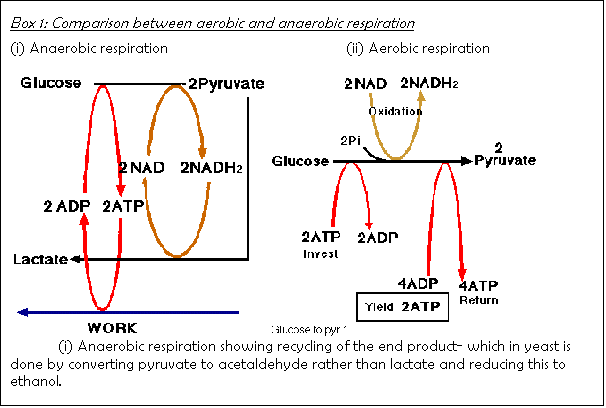 are usually ethyl alcohol and carbon dioxide,
as in yeast cells, or lactic
acid, as in muscle cells.
Another difference between the two methods of respiration is the amount
of energy released. In aerobic
respiration, 32 ATP molecules of energy are released per glucose molecule (see Figure 1). In anaerobic respiration, only two ATP molecules of energy are
released for each glucose molecule.
As the oxygen supply starts to fall
short of the demand by the increasing population, it is less easy for the yeast
cells to oxidise the ethanol and this collects as a toxic by-product of
anaerobic respiration. If left for long
enough, this would in the end caused a rapid decline in the population because
as the oxygen in the solution is used up, the level of ethanol will increase
with the population, and, with time, will reach a level of toxicity where it
actually kills off the population.
Transport of Glucose into Cells
In order to understand how glucose is transported into the yeast cell, it is necessary to study glucose and the barrier that it has to cross, the outer cell membrane, as well as the implications of this.
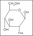 Glucose
The structure of glucose is shown on the right. The many hydroxyl (OH) groups present result it being very polar. It is therefore only soluble in polar substances such as water. It will not dissolve in non-polar hydrophobic environments.
The Fluid Mosaic Model of the phospholipid bilayer
Biological membranes
are bilipid layers. Lipid bilayers are
fluid, and individual phospholipids diffuse rapidly throughout the
two-dimensional surface of the membrane.
This is known as the fluid mosaic model of biological membranes (fluid
because the molecules move around, mosaic because it includes proteins,
cholesterol, and other types of molecules besides phospholipids). In a real cell, the membrane phospholipids
create a spherical three-dimensional lipid bilayer shell around the
cell.  However,
they are often represented two-dimensionally as:
Each ![]() represents a phospholipid. The circle, or head, is the glycerol and
negatively charged phosphate group and the two tails are the two highly
hydrophobic hydrocarbon chains of the phospholipid. The tails of the phospholipids orient towards each other creating
a hydrophobic environment within the membrane.
This leaves the charged phosphate groups facing out into the hydrophilic
environment. The membrane is
approximately 5 nm thick. This bilipid
layer is semi permeable, meaning that some molecules are allowed to pass freely
(diffuse) through the membrane. The
lipid bilayer is virtually impermeable to large molecules, relatively
impermeable to small polar molecules and charged ions, and quite permeable to lipid
soluble low molecular weight molecules.
Its substantial permeability to water molecules is not well
understood. The lipid bilayer is
impermeable to medium and large-sized polar molecules. These molecules depend on hydrophilic
intrinsic protein channels to assist their transport across the barrier by a
process called facilitated diffusion.
represents a phospholipid. The circle, or head, is the glycerol and
negatively charged phosphate group and the two tails are the two highly
hydrophobic hydrocarbon chains of the phospholipid. The tails of the phospholipids orient towards each other creating
a hydrophobic environment within the membrane.
This leaves the charged phosphate groups facing out into the hydrophilic
environment. The membrane is
approximately 5 nm thick. This bilipid
layer is semi permeable, meaning that some molecules are allowed to pass freely
(diffuse) through the membrane. The
lipid bilayer is virtually impermeable to large molecules, relatively
impermeable to small polar molecules and charged ions, and quite permeable to lipid
soluble low molecular weight molecules.
Its substantial permeability to water molecules is not well
understood. The lipid bilayer is
impermeable to medium and large-sized polar molecules. These molecules depend on hydrophilic
intrinsic protein channels to assist their transport across the barrier by a
process called facilitated diffusion.
Facilitated Diffusion
 Molecules
that can diffuse through the membrane do so at differing rates depending upon
the number of channels available for them to pass through the hydrophobic
interior of the membrane bilayer.
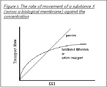
Facilitated diffusion utilises membrane protein channels in the membrane to allow charged molecules (which otherwise could not diffuse across the cell membrane because it is non-polar) to freely diffuse in and out of the cell. These channels are the way in which medium-sized polar molecules like glucose may pass into the cell. The number of protein channels available limits the rate of facilitated transport, whereas the speed of diffusion is dependent only on the concentration gradient. This means that there is a limit to the rate of reproduction of yeast cells, even in ideal circumstances, determined by the rate of facilitated diffusion (see Figure 2). The mechanism is not yet fully understood.
The Reproduction of Yeast Cell
 The way in which yeast cells reproduce also
has an effect on their rate of reproduction.
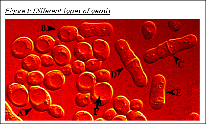
Figure 3 shows the two most commonly studied yeast species, namely budding yeast Saccharomyces cerevisiae (see A and B) and fission yeast Schizosaccharomyces pombe (see C, D, and E).
Budding yeasts (the ones that I will be using) have an oval shape. They multiply by forming buds, which grow in size, and, finally, pinch off from the mother cell. The digestive organelles, called vacuoles, can be identified inside the cells (see F).
Fission yeasts are the rod-shaped ones. They form a septum in the middle of the cell (see C and D) and divide evenly.
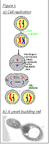
Figure 4 a) shows the basic stages of cell replication. The budding cell is the same size as the original for simplicity. The actual shape is shown in Figure 4 b). The chromosomes replicate themselves and then position themselves with their centromeres attached to the spindle. Their copies then separate and move along the spindle to the polar body on opposite sides of the cell. The bud vacuoles and bud organelles start to form and cytoplasmic division can then take place.
 This is what I expect to happen in terms of
population. At first when the yeast
cells are put into the glucose solution, they take a while to acclimatise. They
may have to produce the RNA to produce the right enzymes, or take a while to
reach to the reproductive stage in their cell cycle.
This is called the lag phase. Once they have done this, the rate of increase in population should get greater as the population of cells increases. This is because if each cell reproduces at a certain rate, the more cells there are, the greater the total rate of reproduction.
However, there are plenty of reasons why the population may not reproduce to its full capacity.
A constant doubling time is a sign of a culture that is growing without constraints like low temperature, lack of food, space or water and without the accumulation of waste products.
Population Dynamics
Here is my mathematical explanation of population growth
Suppose that the culture is not significantly depleting its nutrient reserves or, more accurately, that progress through the cell cycle rather than nutrient uptake is rate limiting. Then the mean reproduction time in this first stage of population growth should be constant for any cohort of cells. Adding glucose would ensure that cell cycle progress continues to be rate limiting until space becomes a limiting factor. The equation for the population is just:
dN/dt=rN((K-N)/K)
Where r is a constant (the intrinsic rate of increase, i.e. the number of reproductive events per unit time per yeast cell), t the time they have been multiplying for, K the maximum number of individuals that the particular environment can support and N is the yeast population number. The solution to this equation is
((K-N)/K)N = N02(t/T)
Where T is the doubling time (normally quoted as 30-60 minutes in ideal conditions) and N0 is the population at time zero. The introduction of K into the equation means that the effect of the environment in slowing down growth to a steady state (or decline) is taken into account. K is also described as the carrying capacity for the environment.
If N>K, growth rate is negative. If K>N, graph of rate is positive, therefore population size tends to settle out at around K=N, that is, population size adjusts to the carrying capacity of the environment. When K=N, the population growth rate is zero. Population size becomes stable. This produces an exponential curve, which levels off, as shown in Figure 5.
However, when a biotic or abiotic factor limits the size of the population, either by two putting limits on the sustainable limits or by slowing down its growth through increased death rate, the exponential increase curve of the population size curves off to a pattern in a fairly short time and can continue in this stable phase for a fairly long time. The factor that causes the eventual decline of the population can be a variety of things: a rapid change in the anaerobic conditions, a build up of toxins produced by the organisms themselves or the introduction of a new predator or disease etc.
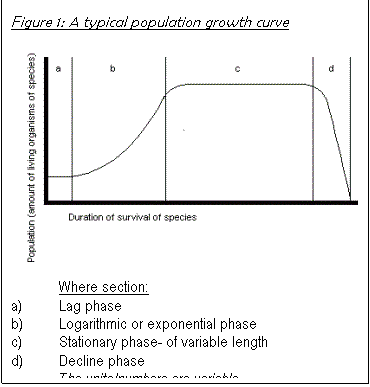 This would produce a population curve
throughout the duration of existence of a species (for a simple case like the
one if we are looking at) that looked something like Figure 5.
This graph only applies if the number living organisms are counted (and not only the number of the cells in a solution) because, for example at stage c), cells are still being produced, its just that the mortality rate is equal to the natality rate but the total number of cells (live + dead) in the solution will still be increasing.
Summary
This is a summary of all evidence so far collected to support a prediction.
1.
Yeast cell respiration
Yeast cells require glucose for metabolism. They respire it anaerobically, then oxidise the ethanol produced. Lack of oxygen causes the build-up of toxic ethanol, which can lead to their death. The larger the population, the greater an effect this will have, leading to the population levelling out as mortality rate increases to mortality rate. This causes the transition from the exponential phase to the stationary phase.
2.
The phospholipid bilayer
Yeast cells gain glucose from the medium in which they are suspended, and because glucose is a polar molecule, the rate of its transport across the membrane depends on the availability of hydrophilic protein channels. An increase in glucose concentration has less of an effect at higher glucose concentrations. Therefore, when the rate of reproduction relies on rate of diffusion, it follows the same trend with concentration as facilitated diffusion does.
3. The reproduction of yeast cells
The rate of reproduction can be limited by progress through the cell cycle (in the lag and exponential phases) or, if the level of glucose is low enough, can be limited by the rate at which glucose can be obtained. A higher glucose level could therefore increase the rate of reproduction.
4. Environmental constraints on the population
These, strictly speaking, should include availability of oxygen and glucose and the build up of toxins. Their effect is the same: when the number of yeast cells is sufficient, they have the effect of either putting constraints on the size of the population, or increasing the mortality rate to the natality rate. The effect of either is the levelling-off of the [living population]-[time] graph. A limitation to the experiment arises if one of these other than glucose concentration affects the population growth rate.
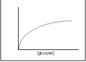 Prediction
During the times for which I plan to run my experiment, I only expect to see the period from the lag phase to the end of the exponential phase. Not many cells will be dying during these initial phases (although possibly a few during the lag if they do not successfully adapt), so the total count will be approximately equal to the living population. The rate of growth will therefore follow the pattern:
Plan
This is the experimental procedure that I plan to follow when I carry out the practical experiment. It is in chronological order. Decisions are backed up with reasoning.
Apparatus:
10 x 100 cm3 conical flasks with cotton wool plugs
Haemocytometer slide with cover slip
1ml teat pipette
Stop clock
Water bath
25 cm3 and 50 cm3 glass pipettes with rubber bulbs
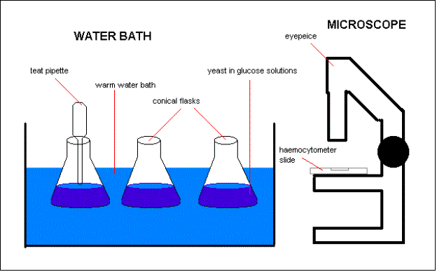 Diagram:
Chronological order of experiment
1) Set up the apparatus as shown above
§ The water bath should be at 40 degrees C (313K)
§ The stop clock should be able to measure hours
2) Put 70 ml of glucose solution in the 100cm3 conical flask
§ This solution is made by simple dilution
§ Use a Burette for this
§ The concentrations that I will use are:
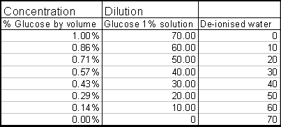
3) The controls that I will use for this experiment are water (de-ionised), glucose and yeast cells that have been subjected to boiling hot water.
4) Leave the solution in the water bath to warm up for 10 minutes or until it is at the same temperature as the water bath
5) Put 1ml of yeast solution into each conical flask
§ Swirl the container that the yeast solution is in before taking any out in case it has settled
§ This should be freshly made 1% solution
§ Use a 1ml pipette
§ Is a sample will need to be accurately diluted for this
§ Check and note down the actual temperature of the glucose solution before adding the yeast solution in the table above
§ Start the stop clock at beginning
§ Put cotton wool plug in
6) Extract a 1ml sample using a pipette
§ Use a 1ml pipette
§ Do this after 24hrs and 48 hrs,
7) Count the yeast cells and calculate their concentration using a the haemocytometer:
I. Make sure both the slide and the cover slip are dry and clean
II. Place cover slip on the middle of the slide, making sure it is lengthways on so that the are longer side of the cover slip is parallel to the long this side of the slide
III. Press they cover slip on to the slide of the haemocytometer until rainbow coloured “Newton’s rings” form
IV. Place the slide under a microscope and focus the microscope so that the detailed part of the grid (square type A) can be seen clearly in the middle- see Figure 6.
V. Place drop of the sample solution in the one of the grooves sticking out from under the cover slip, on the side on which the cells are going to be counted
·
 Count
the number of cells in 6 of the 25 grids (B-type Squares (the grids with three
lines around them- see Figure 6))
in the main area (A-type Square) and divide this by six
· Don’t count B-type Squares with larger than seven in
· Count cells from top left C-type Square (see Figure 6).
· Count the C-type Squares in the B-type Squares line by line, as you would read a book.
· Count the six B-type squares in the A-type Square in the same way.
· Count budding cells that can be seen as two lobes as two cells.
· Record the tally of cells per line of C-type cells
VI. This is the number of cells in 0.004mm3 of the solution
VII. Wipe haemocytometer slide with cotton wool soaked in ethanol (evaporates quickly) in-between use and check for contamination before next and every use.
8) Multiply this by 1/.004 (or by 2.5 and move the decimal place 2 places in this directionà)
· This is the amount in 1 mm3 and can be calculated later
9) Compare this to the original value found in step 2)
10) Calculate K for that concentration and fill this in on the table
· The equation is: K =(2/(c24 /c48)*60*60*4*12)/100000
· Where c24/c48 are concentration of cells after 24 hours/concentration of cells after 48 hours (measured in cells/ml. These are calculated in step 8)
· This can also be calculated later
· This calculates the doubling time in 105 seconds.
11) Run one additional experiment with 0.57143% (30/40) glucose, taking a cell count every thirty minutes. Record the results for this in the time/population table
Reasons for apparatus
These are the explanations for each choice made above.
1)
100cm3 conical flask with cotton wool plug
I chose this because it holds larger volume than a test tube/ boiling tube and sits easily in the water bath. The cotton wool plugs prevents gas exchange.
2)
Haemocytometer
This is the most accurate way of measuring cell content of the solution: actually counts the number one in a precise volume. Other methods of population measurement would be: density of solution, change in mass and changes in the acidity of the solution due to increase in carbon dioxide concentration. These are all indirect ways of measuring population growth. The haemocytometer method actually measures the amount of yeast cells per unit volume. It also involves taking a small sample out, rather than having to measure the mass/density of the whole solution, which would mean removing the entire experiment from of the water bath, which would disrupt the rate of or reproduction.
3)
Slide with cover slip
The cover slip makes sure that the correct volume is on the slide and that the cells are visible (in focus).
4)
1ml pipette
This is most accurate for measuring out the 1ml of yeast solution needed. This is because it is graduated to a higher degree of accuracy than a wider measuring vessel could be - if the lines are closer together it is harder to get the level in the pipette exactly right and if the same difference in height corresponds to the smaller volume, the effect of human error is reduced. This reduces the percentage error for yeast solution added
5)
Burette
Burettes are very accurate for the same reason as explained above. It is also very easy to adjust to the height/volume of the liquid using the rubber bulb and valves at the top. This means that the measurements will be to a higher degree of accuracy, which in turn reduces the percentage error.
6)
Stop clock
This is to make sure that all the times are correct therefore no guessing or estimation
Also it can be stopped and the time that the sample is removed from the culture and it can be checked later after one has concentrated on the cell count.
7)
Water bath
This is to keep the solution at a constant temperature and to optimise the temperature for of the yeast cells to reproduce so that the limiting factor is the glucose concentration.
8)
Concentrations using ratios
This enables me to easily gain highly accurate dilutions of my glucose solution because it to eliminates human error due to taking measurements beyond the accuracy of the measuring vessels or the human eye or using several measuring vessels. The percentage concentrations are irrelevant as these can easily be plotted on a graph afterwards and change anyway when the yeast culture is added. This will reduce the percentage error.
Fair Testing
This is the summary of the steps that I will take to ensure that this is a valid scientific experiment.
Ø Keep the temperature constant by using a water bath at 30ºC
Ø Check the actual temperature with a thermometer and record on table
Ø Use ratios for my dilutions
Ø Use a haemocytometer because it is the most accurate method of measurement known to me
Ø Count the number in five different squares of the main grid on the haemocytometer slide and average them
Ø Do a base count to check the concentration of the solution with which I start.
Ø Use pipettes just large enough to hold the quantities that I am at measuring to reduce the percentage errors
Ø Use a stop clock to ensure accurate timing
Ø Use 70 millilitres of glucose solution so that the dilutions are easy and the samples large enough to sufficiently reduce the percentage error.
Ø Plug the conical flask so that the rate of respiration is not relative to the rate of diffusion of oxygen into the solution, but rather that the gases diffuse at a constant rate
Analysis of results
This is what I will do with my results and how I will record them.
I will record my results in Table 1, shown overleaf.
These are the calculations required to fill the table in:
· Averages: sum of entries/number of entries
· Glucose concentration: [glucose]/total volume in beaker x100
· Concentration of cells per cm3: [average cells per B type square]
· Number of reproductions = [yeast cells] / [yeast cells previously]
2
· Percentage increase: [yeast cells] - [yeast cells previously] x100
[yeast cells previously]
·
Population increase rate: number of reproductions
/ [yeast cells previously]
time taken
I will plot these graphs of my results:
· Population increase every half hour over a period of three hours.
· Initial rate of population increase (R1) against glucose concentration
· Secondary rate of population increase (R2) against glucose concentration
· R1 and R2 against glucose concentration (on one graph for comparison)
· The initial and secondary percentage population increase against glucose concentration
· Comparison graphs for the initial and final percentage increase, and for the initial and final rate graphs
I will also statistically analyse my results using
standard deviation
I will apply this test to each "group" of results I get- i.e. all three repeats of the six readings at each concentration will be analysed together. Spreadsheet's standard deviation and average functions will calculate the standard deviation as a percentage of the average of each group of data by dividing the standard deviation by the mean and multiplying by 100. The formula for standard deviation used is:

Where S = the sum of
n = the number of values
x = a value of the data (the number of cells in a B-type square in this case).
Limitations
These are the factors that I expect to be the greatest limitations on my experiment:
1. Cells dying. This can't be helped and is a limitation because it stops me from counting the actual living population. For the purposes of this experiment to it doesn't matter too much because I will still get a similar increase in population with increase in glucose concentration.
2. The vessel containing the solution. Because these reactions are taking place in heterogeneous state, namely substances in solution reacting, the liquid must be in a container. This in itself is limiting because a population needs space to grow. It is therefore possible that the population will be limited by the space factor therefore resulting in the experiment only being valid for shorter periods of time and lower concentrations. I have tried to avoid this limitation by using a low initial concentration of yeast cells (approximately 0.01-0.02%)
3. Denaturation of the enzymes at high temperatures. This makes it impossible to have a higher temperature than around 40 degrees Celsius. This means that when the other conditions are favourable, temperature could become the limiting factor. I have therefore not used very high concentrations of glucose.
4. Accumulation of toxins. As mentioned earlier, ethanol is produced by the reduction of acetaldehyde. If there is not sufficient oxygen present this will not get broken down and can cause some, and eventually all of the yeast cells, to die. I have avoided this in my plan (to the greatest extent possible) by only running the experiment over a short period.
Precautions
I must take the following precautions during the execution of this experiment:
1. Watch out for parallax error- always take measurements at eye level.
2. Wipe up any spillage immediately after they occur.
3. Check the temperature of the water baths every time I take a sample out and adjust it if it is too high/low.
4. Make sure that I don’t force any more solution out of the bottom of the Burette than naturally drops out when the release valve is open- the Burette is graduated to take the leftover amount into account.
5. Shake the test tubes before extracting a sample to ensure even distribution as the cells may settle out.
Implementing
This section is about my actual practical experimentation.
Modifications
These are the changes that I made to my plan in its implementing:
6. I had to use test tubes instead of conical flasks for incubation of my cultures in the water bath. This was due to the fact that the conical flasks floated.
7. I had to leave extracted samples in the fridge between taking them out of the test tube and doing the cell count because it took so long to count all the cells (approximately three or four hours). This meant that the samples all came out at the same time and stopped reproducing at the same time so the population of each sample remained the same until they were counted. I put all the samples in the fridge at the same time (or at negligible intervals on a scale of 24 hours- 60 seconds) and so they cooled down at the same rate and stopped propagating at the same time.
8. When I checked the samples after 24 hours, they had not increased significantly enough to be sure of a pattern when I checked the percentage increase. I therefore decided to check them again at 72 rather than 48 hours after the cells were introduced. This also reduces the percentage inaccuracies in timing.
9. I found that the population increased too slowly to get results of population increase against time results in three hours. I therefore did not include this extension in the investigation.
Results
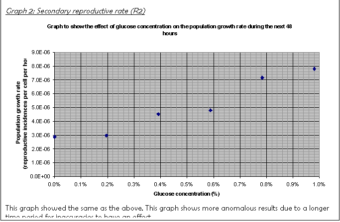
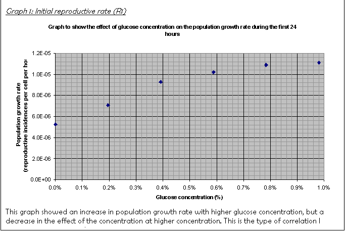 My table of results is on the following page.
The values used for the graphs plotted are printed in
red.
Errors and Limitations
These are limitations or experimental errors that I think have affected my results the most and are responsible for the anomalies pointed out in the next section:
10. Only being able to use 50cm3 in my boiling tubes. The smaller the volume used, the larger the percentage errors are if the measurements are made to the same degree of accuracy.
11. Dead cells. I did not expect the culture to reach the stationery phase and could only tell that it had because of the decrease in rate of reproduction. If I could have measured only the number of living cells, I could have been sure when the culture had reached this stage.
12. Accumulation of toxins. This had an effect because I ran the experiment for 72 hours, by which time the concentration of ethanol had built up to a toxic level.
13. Uneven distribution of cells. Although I shook the test tubes, the distribution was not perfect as the cells clumped together and shaking did not separate the clumps. As these clumps were spread through the solution, the probability of only one or two being in a 0.04 cm3 sample is fairly high, but whether or not there is a clump in the particular B-type square that I count is random, so sometimes there was and sometimes not, leading to huge fluctuations in cell counts.
Anomalies
 The results discussed in the
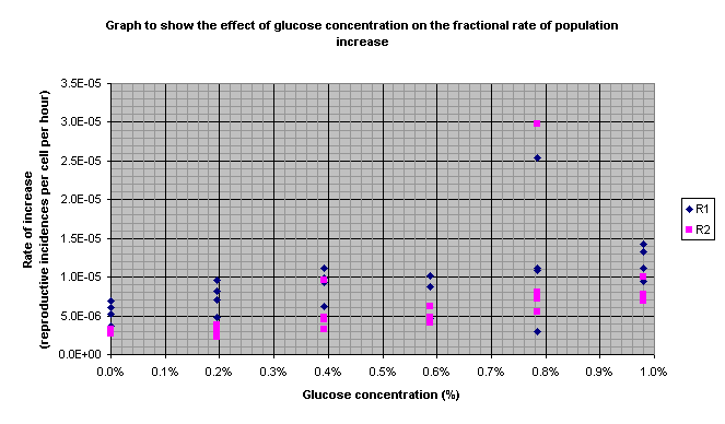
following section seemed obviously faulty. They can be identified on Graph 5
(the highlighted results). The anomalous results were highlighted on the table
and the figures in blue on the table were not included in the calculated
averages. The averages not including the anomalies were then used to plot the
graphs (apart from in the case of Graph 5).
Graph 5
14. The results highlighted in Graph 5 at 0.78% glucose (purple and yellow highlighting on the table)
15. The R2 result above the others at 0.39% glucose and the R1 result below the others at 0.78% (blue numbers on table)
Interpretation of Results
Here are the observations that can be made from the graphs, and a brief explanation of its significance.
16. The graph of R1 (Graph 1) showed that there was already an increase after 24 hours. It showed an increase in reproductive rate with glucose concentration that curved off at higher concentrations. This was only produced when some anomalous results were not included (as explained above). The pattern is explained in the conclusion.
17. The graph of R2 (Graph 2) showed a definite curve of the same type as the R1 graph.
18. 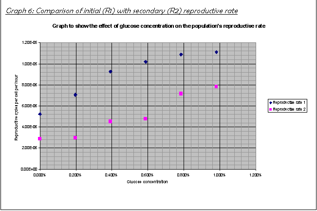 Comparison of R1 and R2 in Graph 6
shows that the population, if at all, only had a short lag phase, in the order
of about 1-5 hours. The population then increased drastically, as Graph 6
shows. The fact that the initial reproductive rate R1 is greater than R2 shows
that by the time I measured the population again at 72 hours after inoculation
shows that the population had already reached the stationary phase by this
time. Therefore, on average over the second and third 24-hour periods, the
population's net increase rate is lower than during the exponential phase. This
is explained more in the conclusion.
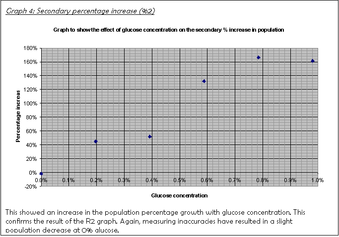
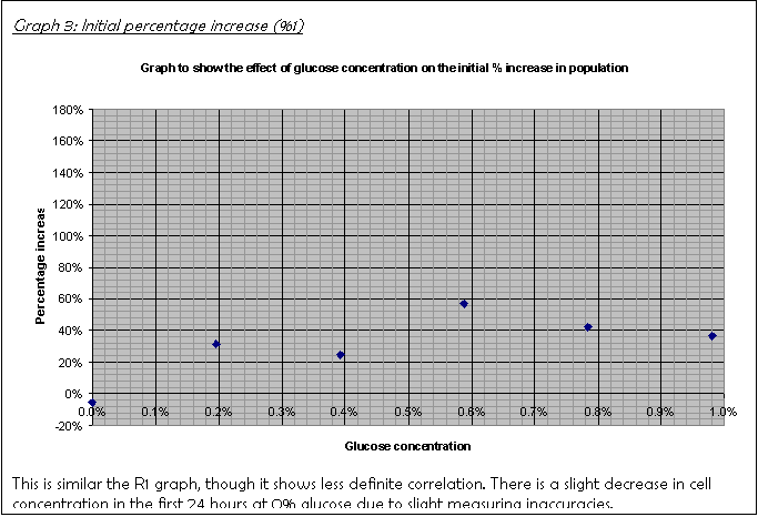
19. Graph 3 and Graph 4 show the percentage increase over the first 24 hours and the next 48 hours, consecutively. A hand-drawn version of Graph 3 was the basis for the decision to leave the culture for another 48 hours rather than just another 24. It did not show a clear trend, which I put down to the fact that the population had not increased sufficiently for the limiting factor to have an effect.
Conclusion
In this section I will summarise what my results show and explain why this occurred. I will then decide whether it matches my prediction.
Summary
- The population had a short lag phase, followed
by a rapid growth phase, then the population slowed down again as it
reached a stationary phase (Graph 6).
For example, compare the growth rates R1 and R2 at 0.98% glucose concentration: R1 is 1.11E-05; R2 is 0.78E-05. The culture slowed down greatly before the time R2 was taken (72 hours after inoculation).
When the yeast culture was introduced, the conditions did not change much from those in the working culture. They may have had to produce the RNA required to synthesise respiratory enzymes to catabolise glucose. As soon as this was done, the cells were in an optimum position to reproduce- the only limiting factor was the rate of progress through the cell cycle. As all the cells can be assumed to be reproducing, the more cells there are at this point, the greater the macroscopic population increase rate. The growth is therefore exponential. As the glucose gets used up, the cells do not receive glucose by diffusion as quickly as before, as the concentration gradient from the medium to the cytoplasm is not as great, and glucose concentration becomes rate limiting. This is explained below. When some cells get no nutrients, they die. The more there are, the more die, so the population plateaus off and a stationary phase begins. See Figure 5.
- The growth was most rapid at the higher
concentrations, and negligible at 0% concentration.
During the exponential phase already, the cultures in the most dilute media will be limited by the rate of diffusion into the cells. The more dilute the solution, the lower the rate of diffusion of glucose into the cell so the slower the rate of reproduction. The populations in the most dilute solutions will therefore increase less rapidly. At 0% glucose the yeast cells had no respiratory substrate so couldn't reproduce.
- The effect of an increase in glucose concentration decreased at higher concentrations.
For example, compare the results for R1: at 0.2% the rate is 7.07E-06, at to 0.39% it is 9.26E-06 whereas at 0.78% it is 1.09E-05, at 0.98% 1.11E-05. The percentage difference between the rates at lower concentrations is much larger than that at higher ones.
Glucose is a polar molecule and is taken into cells by facilitated diffusion. The rate of facilitated diffusion depends on the number of hydrophilic protein channels on the outer membrane. If there is an excess of channels then the rate of diffusion will increase proportionally to the concentration gradient. However, the greater the utilisation of the channels, the more often a glucose molecule will occupy the channel thus preventing a second molecule from passing through. The rate increase with concentration increase therefore decreases as the number of channels utilised increases. The rate of diffusion therefore curves off at higher concentrations. See Figure 2.
Comparison to prediction
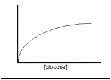 My prediction was: "
During the times for which I plan
to run my experiment, I only expect to see the period from the lag phase to the
end of the exponential phase. Not many cells will be dying during these initial
phases (although possibly a few during the lag if they do not successfully
adapt), so the total count will be approximately equal to the living
population. The rate of growth will therefore follow the pattern:
"
I ran my experiment for longer than I had planned. The culture therefore reached the beginning of the stationary phase. The first sentence was therefore probably a correct estimation. The prediction of the rate of growth in relation to the concentration of glucose was supported by my results. I can therefore conclude that my results did support my qualitative prediction and the rate of population increase does follow the pattern of facilitated diffusion rate.
Evaluation
In this section I will consider the values from the standard deviation test and the number of anomalies, and decide how confident I can be that the results were not purely by chance.
The values obtained are shown on the last column of the table. The greatest standard deviation from the average is 39% at 0.784% glucose. This, however takes the results that I called anomalous into account- hence the high value. Apart from this, the highest value is 30%. This is not very high considering that this is the deviation of the raw data. There were few results that seemed to vary significantly to be recognised as anomalies. These were all mentioned earlier.
More generally, my results are fairly consistent, as well as
being consistent with the prediction, which is an indication that they are
reliable. Some of the finer points of the progress of the population with time
remain to be conclusively proven, but the primary quantitative prediction as to
the effect of glucose concentration on the rate of reproduction appears to be
conclusively and reliably proven.
Hits: