THE EFFECT OF SUCCESSION ON DIVERSITY IN HEATHER MOORLAND

Background Information

In this section I will discuss the factors relevant to the prediction.

Succession

This is the process in which communities of plant and animal species are replaced over time by a series of different and usually more complex communities. It is driven by interspecific competition and an important aspect of it is that at each of the seres until the climax community is reached, populations alter the environment in ways that encourage their direct competitors. The climax community is normally some kind of woodland.

Diversity

This is defined as the number of different species in a particular area.

Heather Moorland

Heather moors are the driest and most widespread of the three types of moorland. They are mostly areas of herbaceous heath* frequently created by the burning down or destruction of woodland (particularly birch Betula and Scots pine Pinus sylvestris) which would otherwise populate the area. They are populated typically by only a few species of heather (e.g. Dorset Heath- Erica ciliaris L., Bell Heather- Erica cinerea L., Common (Ling) Heather- Calluna vulgaris (L.)), mosses (e.g. Feather Moss- Hypnum jutlandicum, Star Moss/Hair Moss- Polytrichum commune) and grasses (e.g. Mat Grass- Narda stricta).

*Strictly this is a misnomer as the dominant heather Calluna vulgaris is an evergreen undershrub, but the term may be conveniently used for areas of low vegetation

This was done primarily for animals to graze on, but nowadays they are valued for their game (grouse). In order to maintain the conditions best suited to heather, and prevent the eventual succession to woodland (e.g. silver birch Betula pendula), it must be periodically (every ten or so years) burned. This has the effect of:

· Burning any developing tree (or shrubs like gorse) shoots (which may be forming due to decline of heather density in the degenerate phase -see below)

· Improving the germination of heather seeds which can benefit from short “heat treatment” and thrive in the moisture- and nutrient-rich blanket

· Increasing the acidity of the soil making it ideal for heather and too harsh for many other plants

Also, after about 15 years, heather's ability to regenerate vegitatively declines and it is therefore necessary to grow new stems, unless heather is to decline.

After the heather is burned, secondary succession occurs. Because heather has the advantages described above, although there may be many species to start with, it takes over eventually as the other plants competing for the same niche are not as successful. The growth phases of Calluna, the primary species, are shown on the left.

After this, the natural series continues with different shrubs like gorses Ulex minor and U. galli colonising the area, and eventually into woodland, probably silver birch Betula pendula.

Prediction

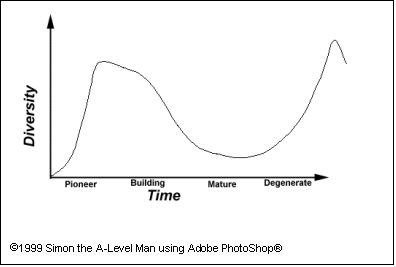I therefore predict that, as succession occurs on heather moorland (see limitation point 3), there will be a fairly short period of high diversity before the heather establishes itself. Then the diversity will fall, as heather's competitors (those species taking up the same niche of the environment) can no longer survive- they are ousted by intraspecific competition. After about thirty or forty years of heather being dominant, if it was left to itself, the diversity would begin to increase again, as heather’s ability to vegitatively regenerate diminishes and a new pioneer community competes to become established. This would at first result in first shrubs and small bushes, then trees and shade-loving plants (as well as many animals), forming a climax community. This can take hundreds of years. However, as the area that I will be studying is still maintained, succession rarely goes further than the mature or degenerate phase, where species number is only beginning to increase again in the form of mosses, grasses and lichens living between heather plants. I have tried to show this pattern on the graph. The drop-off at the end is for the burning of the heather.

Plan

In this section I will detail how I plan to carry out the investigation.

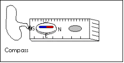
The apparatus

· A point quadrat

· A tape measure

· Plastic tape

· Garden canes

· 1m ruler

· Magnetic compass

diagram of apparatus

Instructions

Basics:

1) Find an area of heather for each of the following (see illustration below):

· Pioneer phase- small pointed plants on freshly burned ground

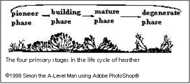· Building phase- heather more mature- heather compact & dome-shaped, less other plants

· Mature phase- high, dome-shaped heather cushions

· Degenerate phase- high, straggly heather with big gaps

2) For each area mark out a square using the measuring tape, plastic tape and garden canes

3) The Quadrat and 1m ruler are then used to sample systematically within the area.

Details:

· 6m*6m area marked out with plastic tape into grid of four 3m*3m areas.

· Samples are taken at the intersections of the tape.

· Use the magnetic compass to ensure that the bar of the point quadrat is in a North-South alignment

· This will give 3*3=9 samples in each area.

· Do this three times for each stage of the heather (pioneer phase, building phase, mature phase and degenerate phase)

· Count multiple hits of the same species with one needle as one hit, for multiple hits of different species with the same needle, count all species hit

· This will give me a total of 3*9*10*4*= 1080 needle readings, and probably many more total hits due to multiple hits

Fair testing

These are the steps I plan to take to make this a valid scientific experiment.

· Keep the samples in each area the same for all samples

· Keep the area the same for all samples

· Use the same quadrat for all samples

· Always use N-S alignment to avoid randomness

· Use systematic sampling to avoid randomness (see below)

Reasoned Explanations

In this section, each decision I have made receives justification.

Point quadrats are more precise than an area quadrat because they count the number of specimens in a particular species, rather than relying on estimates of percentage cover, which introduces human error.

I decided to use 4 different types of sample areas, so that the 4 distinct stages of heather development can be covered.

I used two repeats to ensure incorrect data-, data from an abnormal part of the moor could be identified and ignored, or similar data averaged, and trends recognised.

The tape ensures that the area is big enough for the planned sampling span, and that rows of sampling remain straight. Using a flexible sampling area ensures maximal use of areas, but also that all measurements are within the correct area.

The Simpson Index is an accurate indicator of the relative diversity of areas. It is more accurate than the Simple Diversity Index (the number of differences divided by the total number of organisms), as it accurately takes the size of the individual populations into account

I decided on systematic sampling over random or pseudo-random sampling. As the distribution of species is not simply random, clusters form.

Randomly generated sampling points may be grouped in or around the cluster, therefore not giving a true representation of the data. Pseudo-random co-ordinate generation within the small area that I will be sampling is a waste of time, as it would make little difference on the results.

Diagram left: plants form clusters within a population. Random sampling may coincide with the clusters to produce misrepresentative results.

Analysis of results

This section describes how I will handle and analyse the results.

Recording

Table for my results

The codes for the table are as follows:

· Ecological Stage

Pioneer, building, mature, degenerate

· Species

Number used for reference

· Plant Name

Normal name used for plant

· Species name

Binomial classification (Latin Genus and species)

· Tally 1, 2, 3

Tally of number of hits at site 1, 2, 3

I will record my results in this table:

[Copy of table to be inserted here. The data-collecting table can now be viewed as a web page]

Analysis

These are statistical techniques which may be applied to analyse the results, and their validity.

Diversity: The Simpson Index

From my results, I will calculate the diversity index for each area, and that for each one's average number of species.

The diversity index I decided to use is the Simpson Index.

This diversity index is calculated by:

D= N (N-1)

Σ n (n-1)

Where: D= Diversity index

N= total number of plants

n= total number of individuals of each species

Σ= “sum of“

High diversity index values indicate a large range of organisms in the area of study. This normally occurs in stable ecosystems. Unstable ecosystems or those under stress from pollution or other form of human interference or extreme weather conditions normally have a low diversity index due to large numbers of a few species.

I will represent the diversity index graphically and use this to compare the result with my prediction.

Statistical Tests

These are the statistical tests, which I will carry out on my data to check its validity and bias:

· Standard deviation

· Chi-squared test

This is how I will do them:

Standard Deviation

This is used to analyse the validity of the results. The greater the standard deviation of a set of data, the less valid the mean value is.

The equation for S.D. is:

Where: σ= standard deviation

Σ= “the sum of“

d² = the individual values of d, the diversity index, squared

D²= the mean of the values of d (the sum of them divided by the number of them), squared

n= number of values of d in the data

Therefore the standard deviation is the route of ((the sum of all values of x² minus the mean of x²) divided by n, the number of values of x in the data).

The Chi-squared test

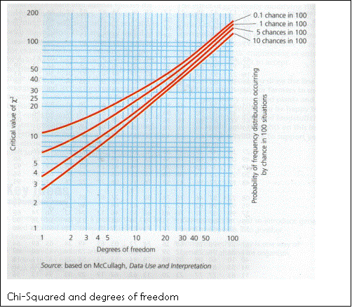This can be used to analyse results for evidence of linkage (positive/negative ecological association).

The equation is:

Where: x²= Chi-squared value

Σ= “sum of“

O= Occurrence of one species together with another

E= Expected value for the latter (calculated by simple probability- if one species occurs 75% and another 50% the occurrence together would be .75*.50=37.5%)

The degree of freedom (df) value must then be found by n-1, one less than the number of samples taken, and the approximate association probabilities can be read off from this graph:

Limitations

These are factors that limit the validity of the experiment, but are for the most part unavoidable.

Random errors: Varying abiotic factors

Wherever this experiment is done, it will not be a perfect representative of “heather moorland”, due to environmental variation. This is because different areas are subject to different conditions and therefore different ecological pressures acting on succession. The three specific problems (limitations) that could affect my results:

· Varying abiotic factors which will cause species distribution variation from site to site on the moors:

Ø pH- affects how many types of plant can grow there

This is related to formation rate, depth and mineral content of the peat. Low pH favours bilberry Vaccinium myrtillus

Ø Gradient- affects water runoff

Ø Depth of peat- affects water retention and therefore availability

Boggier conditions favour Spaghnum sp. moss, thinner layer of bog causes heath-like condition, and deeper peat favours bilberry Vaccinium myrtillus

Ø Aspect- affects temperature and light

Ø Height- affects temperature, exposure, moisture and light

Bilberry Vaccinium myrtillus is more tolerant to both exposure and shade so often dominates higher zones (up to 1300m in Britain), and Vaccinium ugliginosum slightly below this level (Northern Europe)

Ø Topography- affects wind speed

Exposure to high wind speed causes the rapid loss of water. These conditions favour plants that can survive well in dry climates. This is why, despite the water-logged soil, the plants on moorland appear to be well adapted to a dry environment, as non-xeromorphic plants might be expected to lose water rapidly by transpiration (also see below).

Ø Sand/air content of peat

The rate at which plants take up acid water through their root systems tends to be reduced when the supply is cold and low in oxygen

The important fact is that the above factors, and others, cause different degrees of environmental resistance acting on different species, depending on their sensitivity to the factors, and their particular optimum conditions. Therefore, the change in environmental conditions between specific patches of the moor causes a difference in which species are favoured more by the environment in each particular spot.

Systematic errors: human influences

Because of the nature of the experiment (investigation a specific type of area), the areas investigated need to be chosen and not systematically or randomly picked from a map. This introduces bias into the results e.g. might pick area with prettiest flowers therefore lots of bell heather in results!

· Another limitation is that the three types of moorland, namely heather (heath), bilberry and cottongrass (bog), merge into one another and co-exist. The result of this is that, especially in an area of pioneer or building phase heather, the results may vary greatly, or give a false indication of diversity as an average, as the patches which can be separately defined as heather moor are so small. If we were to ‘avoid’ this limitation by only choosing sites that showed a high proportion of heather, we would have the problem they would be non-comparable, as they would all have a low level of diversity due to the reason for their selection!

Precautions

These are the precautions I shall have to take during the execution of the research:

· Use compass for N-S alignment of quadrat

· Analyse the data “out in the field” to check validity and modify method as necessary- e.g. if the variation of averages of the three sets of data in the same type of area is much greater than about 5%, the sample areas aren’t big enough.

Modifications

During the conduction of the practical experiment, I made these modifications to my method:

· I discovered that, as the species present and therefore ecological associations present vary greatly according to the phase of heather, the Chi-Squared test could not be used across all my results. Too few of the species were abundant enough in all phases for a survey of this size to collect enough data about enough species to warrant using this analysis method, as the test requires large amounts of data to be valid. I therefore will not analyse the data by these means.

· Heavy rain prevented the detailed statistical analysis of results (using a calculator) in the field, and the method was therefore adapted as described below to ensure best use of the available sampling areas.

· I varied the sizes of my sampling areas to fit into the various size areas of suitable heather- e.g. square approximately 50*50 into an area of 75m radius. For the quadrat spacing I divided the length of the side of the square by three to give the spacing x. I then took three samples along row A (through the middle of the square area, perpendicular to one side), distance x apart. I did this again distance x away from and parallel to row A on either side of it to form a grid. This still gave 3*3=9 samples in each area.

Results

Notes on the results

Ø The error bars on the average values for diversity on the graph “SIMPSON INDEX (ALL DATA)” are for 30% variation. Value labels are for the diversity index number of the average.

Ø The “misses” values have, of course, not been used to calculate diversity, but merely exist for evaluation purposes.

Ø For each experiment on the “Results Table”, I have calculated

o (n1)*((n1)-1), or the number in sample (n) multiplied by one less than n. “n1” corresponds to the number in sample 1, “n2” to that in sample 2, etc. Henceforth I will refer to the n for any sample x as “n_x”. This calculation is necessary for the diversity index calculation.

o The total of the above values, Σ n_x (n_x-1) for the diversity index calculation.

o The total of the values of n_x, N.

o The diversity index, d, for each: sample 1, 2, 3: - d₁, d₂, d₃, and the diversity of the averages, d_a.

Ø “Species” 1, 2, 3 etc. refers to the number denoted to these species in the table constructed to collect data in the field.

the results

Big table

[Page with table to be inserted here]

Main graph

[Page with diversity graph to be inserted here]

The table and graph can be viewed as a web page if you click here.

Conclusion

These results show that, as I had predicted, the diversity index value dips as the heather matures, then rises again as it becomes degenerate.

The linear representation of the averages (SIMPSON INDEX (ALL DATA) graph) of the values collected in the field shows a similar trend to that predicted. This is because, as heather matures along with other species in the same niche of the environment, the competitive exclusion principle predicts that, due to differential resource competing ability, only one will be successful. Heather moorlands are merely areas where the sum of the biotic and abiotic factors (environmental resistance) favours Ling Heather Calluna vulgaris and Bell Heather Erica cinerea. Other types of heather like Cross-leafed heath Erica tetralix and Dorset Heath- Erica ciliaris L. can also be present, but they did not occur in my samples. As the definition of heather moorland given at the beginning is that it exists only in an era shortly following the burning of the area, add the fact that Calluna passes it’s prime after a certain length of time, and it is only natural that the beginning and end of the cycle are high diversity. For example, the average diversity index value during the pioneer phase is 4.5, during the building phase 3, during the mature phase 2, and during the degenerate phase 7.3.

Discussion

The degree to which errors, anomalies and limitations affected my results

Statistical analysis of results using Standard Deviation

x, the number of values of d, is always 4.

For the Pioneer phase:

Standard deviation calculations
Numbers	dx	dx^2
1	4.879	23.80257
2	2.555	6.530538
3	2.468	6.091217
a	4.516	20.39125
Total (Σ)	14.418	56.82
Average	3.604497
Average squared (D^2)		12.9924

S.D.= 3.31

For the building phase:

Standard deviation calculations
Numbers	dx	dx^2
1	1.810	3.275297
2	2.819	7.947449
3	4.259	18.13983
a	3.042	9.253363
Total (Σ)	11.930	38.62
Average	2.982481
Average squared (D^2)		8.90

S.D.= 2.73

For the mature phase:

Standard deviation calculations
Numbers	dx	dx^2
1	2.808	7.883221
2	1.579	2.494802
3	1.667	2.779649
a	2.044	4.177147
Total (Σ)	8.098	17.33
Average	2.024559
Average squared (D^2)		4.10

S.D.= 1.82

For the degenerate phase:

Standard deviation calculations
Numbers	dx	dx^2
1	5.915	34.991
2	8.541	72.95384
3	6.803	46.2758
a	7.308	53.41213
Total (Σ)	28.568	207.63
Average	7.141903
Average squared (D^2)		51.01

S.D.= 6.2

The reason behind the fluctuation occurring with a similar pattern to the diversity index number could lie in the fact that as diversity decreases, it becomes much easier to pick out similar sites. This is explained more fully below:

It gets easier to pick out sites that are close to the definition of “heather moorland” at the more mature phases of the heather, but before it becomes degenerate, because by this time, if present, Calluna becomes either very dominant or scarce. As the sites become easier to pick out, because it is obvious when if don’t fit the definition the definition, less and less results deviation can exist. Where there is a higher diversity, results could (for example in the pioneer phase results) include:

· bog gaining a covering of heather as it dries out

· bilberry moor with heather taking over

· freshly burned bracken moor with heather regenerating vegitatively taking advantage of nutrients and making shoots before bracken takes over again

or similar, for the same phase. Therefore, the results would deviate a lot, although the landscape of the area covered with the new (pioneer phase) heather would look similar in all these situations.

Limitations

This shows that the limitations affected my results to a lesser or greater degree, but if interpreted as above, this could strengthen my conclusion.

The particular limitations that affected my results are probably:

· Human bias is introduced through the need to investigate a specific type of area requiring the areas investigated to be chosen and not systematically or randomly picked from a map (e.g. choose area nearest to road, which may not be the best representative of the phase).

· This causes problems because the variation of environmental (abiotic) factors* causes species distribution variation from site to site on the moors, so no two areas are the same.

* These include the depth of the peat, gradient and aspect of the slope on which the sampling site was situated, height and topography of the terrain and nutritional qualities of the peat.

· The above is due to the different degrees of sensitivity and spectrum of tolerance of different species and the change in environmental conditions between specific patches of the moor, so that the environments of different sites favour different species. One patch of degenerate phase heather, for example, may be less diverse than another, due to being in a more exposed situation. The patches of heather in different situations may be surrounded by a different enough community to be classed as a different type of moor, but the three types of moorland, namely heather (heath), bilberry and cottongrass (bog), merge into one another and co-exist.

· This resulted in the great degree of variation, especially in the pioneer and building phase samples. They could have given a false indication of diversity as an average, as the patches which could be separately defined as “heather moorland” were so small, that sometimes the sampling area may have included pockets of bog or bilberry moor.

Errors and Anomalies

The limitations on this experiment resulted in a general tendency for large degrees of variation. It is therefore difficult to pick out any individual anomalies. Any particularly large differences are picked out on the results sheet using a highlighter. The values are quoted as they appear on the table: experiment 1 value, experiment 2 value, experiment 3 value e.g. Plant x: 5, 7, 15 means 5 hits (of this plant) for experiment one, 7 hits for experiment two, and 15 hits for experiment three.

Pioneer: Experiment three in the pioneer phase shows that a different type of area was being sampled to the other two surveys in that phase e.g. 61, 41, 0 for Calluna and 7, 3, 35 for bracken. Heath rush Funcus squarosus varies greatly too: 20, 0, 0. The fact that the diversity values of experiments 2 and 3 are at all similar may be seen as surprising. Experiments 1 and 2, however, are similar terrain, and have quite different values. Discounting experiment 1 on the grounds of its very different diversity index would result in a very low average. This could be due to very harsh conditions very shortly after burning, but is not normal. Discounting experiment 3 as the plants present are so different would result in a greater average diversity value.

Building: The results for this phase are fairly consistent between experiments 1 and 2, but 3 tends to be different. e.g. Calluna 83, 72, 34 and Funcus 9, 6, 21. The average without experiment 3 would be lower.

Mature: Here all the experiments are very similar e.g. Calluna 66, 75, 77, apart from crowberry Empetrum nigrum 25, 0, 0, with the resulting higher diversity for experiment 1. Ignoring experiment 1 would result in a lower value.

Degenerate: This showed more general variation e.g. Calluna 58, 34, 41, bilberry Vaccinium myrtillus 51, 20, 35, mat-grass Nardus stricta 14, 25, 16. Experiment 2 appears the oddest one out.

Overleaf is shown the resultant graph missing out the experiments shown in this analysis of anomalies to be slightly misfitting. The trend is not changed, it is merely accentuated. I therefore think that with the number of readings that I have taken (1741 hits), the averages should be taken as valid, as, however the limitations have affected the results, the three experiments’ results seem to compliment each other to result in a feasible trend. Because of this I think that there were no significant errors in experimental method, apart from maybe it should have been a bigger survey. This is discussed more below.

Conclusion Evaluation in the light of the errors, anomalies and limitations

As the conclusion is in agreement with scientific principles (the competitive exclusion principle and resource partitioning), it could be assumed valid. The analysis showed that the most consistent results were obtained in those areas where heather grew in its mature phase. The reasons for this are discussed on the previous page. The graph shows that the data did vary quite a lot, as the results are often not even within the 30% error bars. This and the higher S.D. values mean that the value that I obtained as an average is not as valid. I therefore plotted the values without the averages to view the data spread overleaf.

Although the mature phase is overall the lowest and the pioneer phase overall the next, with the degenerate phase having the highest diversity, the values for the building phase stretch from 1.81 to 4.26 (colours correspond to data spread graph). Taking this data into account, we cannot make any real conclusions other than that:

· The pioneer and building phase are of moderate diversity

· The mature phase is of low diversity

· The degenerate phase is of high diversity

This is much in agreement with the graph in my prediction, although the relative values for pioneer and building phase turned out to be lower than I expected. This could be because not as many species as I expected are able to take advantage of the high nutrient environment created by burning the moorland, due to the harshly acidic conditions prevalent in the ash. A reason why heather could become established so easily is that by the time soil conditions are favourable for them, competitors cannot compete, as the land has already been commandeered by heather. Although the individual diversity values seem to suggest unreliable results, the trend of the averages seems to follow logic.

My prediction was more qualitative than quantitative, so I conclude that the principles therein still hold true, but this investigation is not conclusive. A greater number of surveys on each phase could better be grouped in types of moorland (with/without bracken, bilberries etc.), and the trends be analysed to find out if they hold true for all types of areas.

Hits:

References

Name: Author: Publisher:

1. Introduction to Ecology R. Dajoz UNIBOOK

2. Mountains and Moorland A. Darlington George R. Ltd.